From Uniswap v3 to crvUSD LLAMMA|Curve|crvUSD|stablecoin|LLAMMA • 0xreviews.xyz

Origin paper: 《From Uniswap v3 to crvUSD LLAMMA.pdf》

Preface： The most difficult part of Curve stable coin is LLAMMA (AMM for continuous liquidation/deliquidation). LLAMMA refers to some of the principles in Uniswap v3. However, the price in the white paper is different from the mathematics in the Uniswap v3 white paper. We will unify these two projects and try to figure out how Curve CEO designed the algorithm.

Refer to Uniswap v3

The definitions of price in this article and Uniswap v3 are reciprocals of each other. Therefore, we have modified the formulas in the Uniswap v3 white paper to make them consistent with this article. In short, LLAMMA tries to make everything dynamic in Uniswap v3 to give a more preferable price for both crvUSD debtors and liquidators.

Compare the constant product formulas

Formula (2.2) from Uniswap v3 whitepaper:

\begin{aligned} (x+\dfrac{L}{\sqrt{P_b}})(y+L\sqrt{P_a})=L^2 \end{aligned}

Uniswap v3 Simulation of Virtual Liquidity

Formula (1) in the Curve stablecoin whitepaper :

\begin{aligned} I = (x + f) (y + g) \end{aligned}

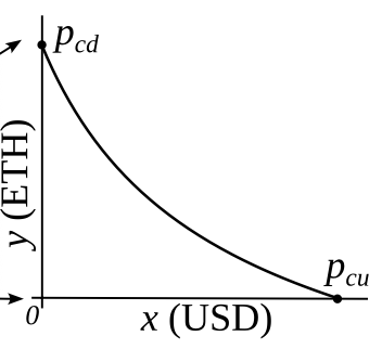
AMM with an external price source

Here $P_{cd}$ means $P_{current\_down}$ , $P_{cu}$ means $P_{current\_up}$ .
The corresponding relationship is:

P_{b} = \dfrac{1}{P_{cd}}, P_{a} = \dfrac{1}{P_{cu}}, L=\sqrt{I}

The corresponding constant product formula is:

\begin{aligned} (x+\sqrt{I}\sqrt{p_{cd}})(y+\dfrac{\sqrt{I}}{\sqrt{p_{cu}}})=I \end{aligned}

Among them:

f=\sqrt{I}\sqrt{p_{cd}}, g=\dfrac{\sqrt{I}}{\sqrt{p_{cu}}}

Liquidity Calculation Formula Correspondence

Formula (6.7) from Uniswap v3 whitepaper:

\begin{aligned} L=\dfrac{\Delta{y}}{\Delta{\sqrt{p}}} \end{aligned}

Because of the reciprocal relationship between their price definitions, it corresponds to the formula:

\begin{aligned} \sqrt{I} = \dfrac{\Delta{y}} {\Delta{\sqrt{\dfrac{1}{p}}}} \end{aligned}

One specific application of this formula is:

\begin{aligned} \sqrt{I} = &\dfrac{(y_0-0)}{(\dfrac{1}{\sqrt{p_{cd}}}-\dfrac{1}{\sqrt{p_{cu}}})} \\ = &\dfrac{\sqrt{p_{cd}p_{cu}}}{\sqrt{p_{cu}}-\sqrt{p_{cd}}} y_0 \end{aligned}

Do square expansion to get:

\begin{aligned} I= \dfrac{{p_{cd}p_{cu}}}{p_{cu}+p_{cd}-2\sqrt{p_{cd}p_{cu}}} y_0^2 \end{aligned}

From the above formulas, we can easily find that when $y_0$ remains constant, The closer $p_{cd}$ and $p_{cu}$ are, the greater the corresponding liquidity $I$ .

In another word:

\lim\limits_{p_{cd} \to p_{cu}} \sqrt{I}= +\infty

The liquidity cannot be infinite, and the corresponding minimum tick in Uniswap v3 will limit the size of $L$ .

From this, it can be deduced that in LLAMMA, we also need to define an indicator to measure the minimum difference between prices, and continue the analogy between Uniswap v3 and Curve.

Correspondence between the minimum price difference

\dfrac{p\downarrow}{p\uparrow} = \dfrac{A-1}{A}

It can be seen from the definition of $A$ , the closer $p\downarrow$ and $p\uparrow$ are, that is, the larger A is, the higher the liquidity concentration:

A = \dfrac{p\uparrow}{p\uparrow - p\downarrow}

In Uniswap v3, only ticks with indexes that are divisible by tickSpacing can be initialized. Thus, tickSpacing determines the minimum price range for LPs to allocate their liquidty. The smaller the tickSpacing is, the tighter and more precise the price ranges. In Uniswap v3 different fee tiers determine different tickSpacing.

However, there is no need for crvUSD LLAMMA to have so many tickSpacing. Just make every $tickSpacing = 100 base point$ since LLAMMA is just for ETH-crvUSD. Formula (6.1) from Uniswap v3:

p_i=1.0001^i

In LLAMMA, A=100, Formula (11) from Curve stablecoin whitepaper:

\begin{aligned} p\uparrow (n) = (\dfrac{A-1}{A})^n p_{base} \end{aligned}

\begin{aligned} p\downarrow (n) = (\dfrac{A-1}{A})^{n+1} p_{base} \end{aligned}

Set $n = -i$ and $A=100$ , we have:

\begin{aligned} p\uparrow (-i) = (\dfrac{100}{100-1})^i p_{base}\ \ \ \ \end{aligned}

Design $p_{cd}$ and $p_{cu}$

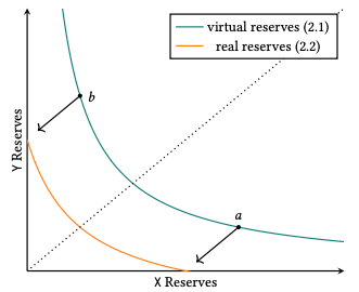
We hope that LLAMMA has the following properties: when the price of ETH rises, the pool buys ETH. When ETH falls, the pool sells ETH. Given this, we define $p_{cd}$ and $p_{cu}$ as functions of $p_o$ and are steeper than linear functions, so their growth rates will be faster than $p_o$ . At the same time, it can be seen from the figure that the two curves $p_{cu}$ and $p_{cd}$ pass through two points $(p\downarrow,p\downarrow)$ and $(p\uparrow,p\uparrow)$ respectively. The $p_{cd}$ and $p_{cu}$ that meet the above requirements actually have many curves. The general formula is:

p_{cd} = \dfrac{p_o^{n+1}}{p\uparrow^n}, p_{cu} = \dfrac{p_o^{m+1}}{p\downarrow^{m}}

where $m<n$ .

Let's start from the simplest case:

p_{cd} = \dfrac{p_o^2}{p\uparrow}, p_{cu} = \dfrac{p_o^2}{p\downarrow}

Substitute $p_{cu}$ and $p_{cd}$ into the square expansion of $I$ :

\begin{aligned} I= &\dfrac{{p_{cd}p_{cu}}}{p_{cu}+p_{cd}-2\sqrt{p_{cd}p_{cu}}} y_0^2 \\ = &\dfrac{\dfrac{p_o^2}{p\uparrow}\dfrac{p_o^2}{p\downarrow} y_0^2}{\dfrac{p_o^2}{p\uparrow} + \dfrac{p_o^2}{p\downarrow} - 2\sqrt{\dfrac{p_o^2}{p\uparrow}\dfrac{p_o^2}{p\downarrow}}}\\ =&\dfrac{p_o^2 y_0^2}{p\downarrow+p\uparrow - 2\sqrt{p\downarrow p\uparrow}}\\ =&\dfrac{p_o^2 y_0^2}{(\sqrt{p\uparrow}-\sqrt{p\downarrow})^2} \end{aligned}

Then $f^2$ can be calculated as:

\begin{aligned} f^2=&Ip_{cd}\\ =&\dfrac{p_o^2 y_0^2}{(\sqrt{p\uparrow}-\sqrt{p\downarrow})^2}·\dfrac{p_o^2}{p\uparrow} \end{aligned}

It is not difficult to find that $f^2$ is hard to comprehend and calculate under this assumption. What if $p_{cd}$ and $p_{cu}$ are cubic functions of $p_o$ :

p_{cd} = \dfrac{p_o^3}{p\uparrow^2}, p_{cu} = \dfrac{p_o^3}{p\downarrow^2}

Substitute $p_{cu}$ and $p_{cd}$ into the square expansion of $I$ :

\begin{aligned} I= &\dfrac{{p_{cd}p_{cu}}}{p_{cu}+p_{cd}-2\sqrt{p_{cd}p_{cu}}} y_0^2 \\ = &\dfrac{\dfrac{p_o^3}{p\uparrow^2}\dfrac{p_o^3}{p\downarrow^2} y_0^2}{\dfrac{p_o^3}{p\uparrow^2} + \dfrac{p_o^3}{p\downarrow^2} - 2\sqrt{\dfrac{p_o^3}{p\uparrow^2}\dfrac{p_o^3}{p\downarrow^2}}}\\ =&\dfrac{p_o^3 y_0^2}{p\downarrow^2+p\uparrow^2-2p\downarrow p\uparrow}\\ =&\dfrac{p_o^3 y_0^2}{(p\uparrow-p\downarrow)^2} \end{aligned}

Recalculate $f^2$ :

\begin{aligned} f^2=&Ip_{cd}\\ =&\dfrac{p_o^3 y_0^2}{(p\uparrow-p\downarrow)^2}·\dfrac{p_o^3}{p\uparrow^2}\\ =&\dfrac{p_o^6 y_0^2}{(p\uparrow-p\downarrow)^2 p\uparrow^2} \end{aligned}

It can be seen that when $p_{cd}$ and $p_{cu}$ are cubic functions of $p_o$ , the whole mathematical form is much simpler. The square root term is eliminated, and the calculation is much more convenient. If a higher order is taken, the price of AMM and $p_o$ will differ greatly, and thus the cost of buying ETH (when the price rises) will be much higher, which leads to a greater loss of liquidation. In summary, it is a better choice to define $p_{cd}$ and $p_{cu}$ as cubic functions of $p_o$ .

Derivation of other parameters

On the basis of assuming that $p_{cd}$ and $p_{cu}$ are cubic functions about $p_o$ , taking the special value $p_o=p\uparrow$ , it is not difficult to obtain that $y=y_0$ and $x=0$ , then:

\begin{aligned} I=&\dfrac{p_o^3 y_0^2}{(p\uparrow-p\downarrow)^2}\\ =&p_o y_0^2 · \dfrac{p_o^2}{(p\uparrow-p\downarrow)^2}\\ =&p_o y_0^2 · (\dfrac{p\uparrow}{p\uparrow-p\downarrow})^2\\ =&p_oy_0^2A^2 \end{aligned}

Given the fomula of $I$ , we can calculate $f$ and $g$ :

\begin{aligned} f=&\sqrt{I}\sqrt{p_{cd}} \\ =&\sqrt{p_oy_0^2A^2}\sqrt{\dfrac{p_o^3}{p\uparrow^2}}\\ =&\dfrac{p_o^2}{p\uparrow}Ay_0 \end{aligned}

\begin{aligned} g =& \dfrac{\sqrt{I}}{\sqrt{p_{cu}}}\\ =& \dfrac{\sqrt{p_oy_0^2A^2}}{\sqrt{\dfrac{p_o^3}{p\downarrow^2}}}\\ =&\dfrac{p\downarrow}{p_o}Ay_0\\ =&\dfrac{p\uparrow}{p_o}(A-1)y_0 \end{aligned}

From this, we finally get the complete constant product formula:

(\dfrac{p_o^2}{p\uparrow}Ay_0 + x)(\dfrac{p\uparrow}{p_o}(A-1)y_0 + y) = p_oA^2y_0^2

Transform the above equation into a quadratic equation of $y_0$ :

p_oAy_0^2- y_0(\dfrac{p\uparrow}{p_o}(A-1)x + \dfrac{p_o^2}{p\uparrow}Ay) - xy = 0

Use the quadratic equation of one unknown to solve $y_0$ :

y_0 = \dfrac{(\dfrac{p\uparrow}{p_o}(A-1)x + \dfrac{p_o^2}{p\uparrow}Ay)+\sqrt{(\dfrac{p\uparrow}{p_o}(A-1)x + \dfrac{p_o^2}{p\uparrow}Ay)^2+4p_oA·xy}}{2p_oA}

If the price moves so slowly that the oracle price $p_o$ is fully capable to follow it, given $x$ and $y$ , using the calculation formula of Uniswap v3, it is possible to calculate how much $y\uparrow$ of ETH (if the price rises) or $x\downarrow$ of USD will eventually be in the band (if price drops):

\begin{aligned} y\uparrow =& y + \Delta y \\ =& y + \sqrt{I}(\dfrac{1}{\sqrt{p\uparrow}} - \dfrac{1}{\sqrt{p}}) \\ =& y + \dfrac{\sqrt{I}\sqrt{p} - \sqrt{I}\sqrt{p\uparrow}}{\sqrt{p\uparrow p}} \\ =& y + \dfrac{(f +x) - f}{\sqrt{p\uparrow p}} \\ =& y + \dfrac{x}{\sqrt{p\uparrow p}} \end{aligned}

\begin{aligned} x\downarrow =& x + \sqrt{I}(\sqrt{p\downarrow}- \sqrt{p}) \\ =& x + \sqrt{I}(\dfrac{1}{\sqrt{p}} - \dfrac{1}{\sqrt{p\downarrow}})\sqrt{p\downarrow p}\\ =& x + ((g+y) - g)\sqrt{p\downarrow p}\\ =& x + y\sqrt{p\downarrow p} \end{aligned}

Reference

[1] Adams, Hayden, et al. "Uniswap v3 core." Tech. rep., Uniswap, Tech. Rep, 2021 from https://uniswap.org/whitepaper-v3.pdf

[2] Egorov, Michael, and Curve Finance. Curve stablecoin design. Technical report, Curve Finance, Tech. Rep, 2022 from
https://github.com/curvefi/curve-stablecoin/blob/master/doc/curve-stablecoin.pdf

From Uniswap v3 to crvUSD LLAMMA